1 Move from simultaneous dropouts to a frequency check

For a quick solution, go to section 3. Imagine four wireless microphones that work individually but drop out when used together. Check the receiver's RF and audio indications first to see whether the fault points toward the wireless link, then examine the channel combination. This article focuses on frequency relationships; simultaneous-operation problems alone do not prove intermodulation.

2 Compare intermodulation with equal and unequal spacing

A scan helps identify signals already present at the venue. Coordination also considers additional frequencies that may arise when equipment operates together. When multiple RF signals enter a nonlinear circuit, sum, difference and other combination frequencies can appear. These are intermodulation products: additional frequency components created by nonlinear behavior, rather than an unexplained extra microphone transmitting at the venue.

Third order does not mean three microphones. In the two-frequency expression 2×B−A, the absolute coefficients add to three. Three different channels can also create third-order products such as A+C−B. The four figures below compare inputs, positions and results using the simulator's default ±50 kHz teaching tolerance throughout. Keeping the same tolerance and calculation types makes the two examples directly comparable.

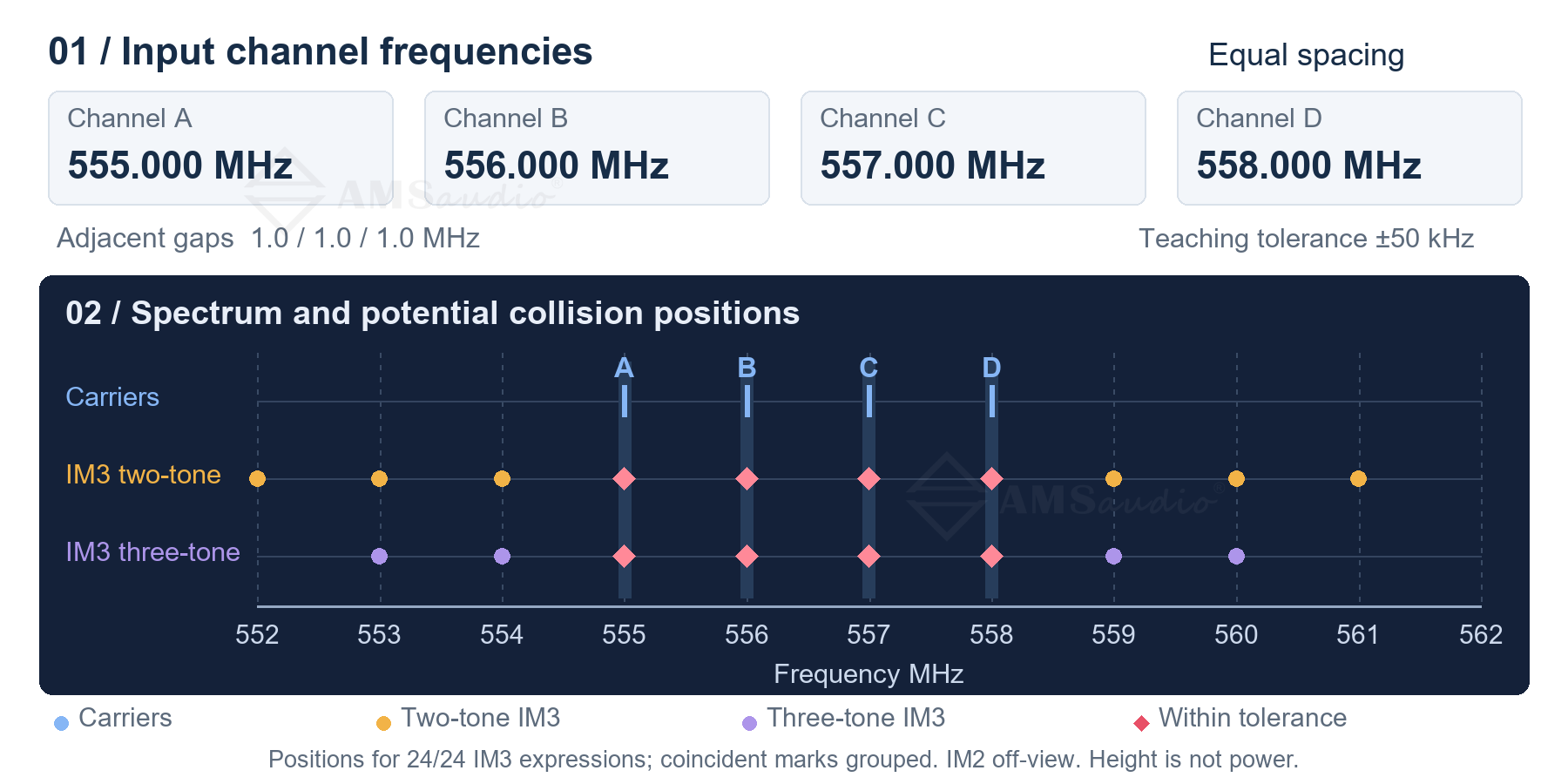
Figure 1  Equally spaced inputs and potential collision positions

The equally spaced group is A=555, B=556, C=557 and D=558 MHz, with a 1 MHz gap between adjacent channels. The expression 2×556−555 gives 557 MHz, exactly at C; 2×557−556 gives 558 MHz, at D. Checking that the four carriers are separate does not check these combination relationships.

Key calculations for the equally spaced group

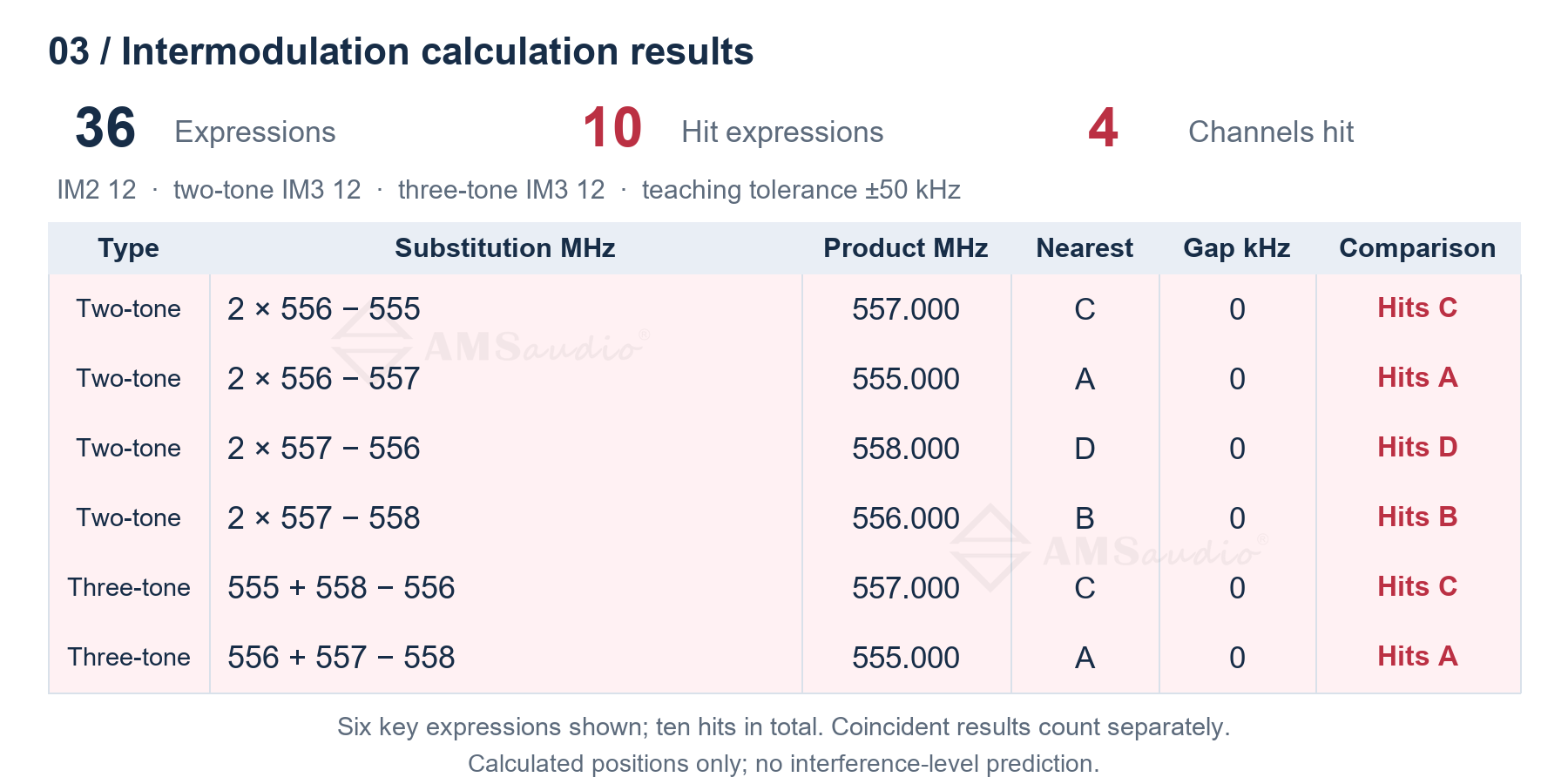
Figure 2  Key intermodulation results for equal spacing

The default model lists 36 expressions: 12 second-order, 12 two-frequency third-order and 12 three-frequency third-order expressions. Ten meet the hit criterion at channels A through D; Figure 2 shows six selected examples. The count is by expression, not by unique frequency. Several expressions can produce the same position, so ten flagged expressions do not mean ten separate interfering signals exist.

How unequal spacing changes the positions

Switch to the simulator's unequal-spacing example: 555, 556.3, 557.9 and 560.2 MHz. The adjacent gaps become 1.3, 1.6 and 2.3 MHz. Keep the tolerance and calculation types unchanged so that the comparison isolates the frequency combination rather than a change in the test settings.

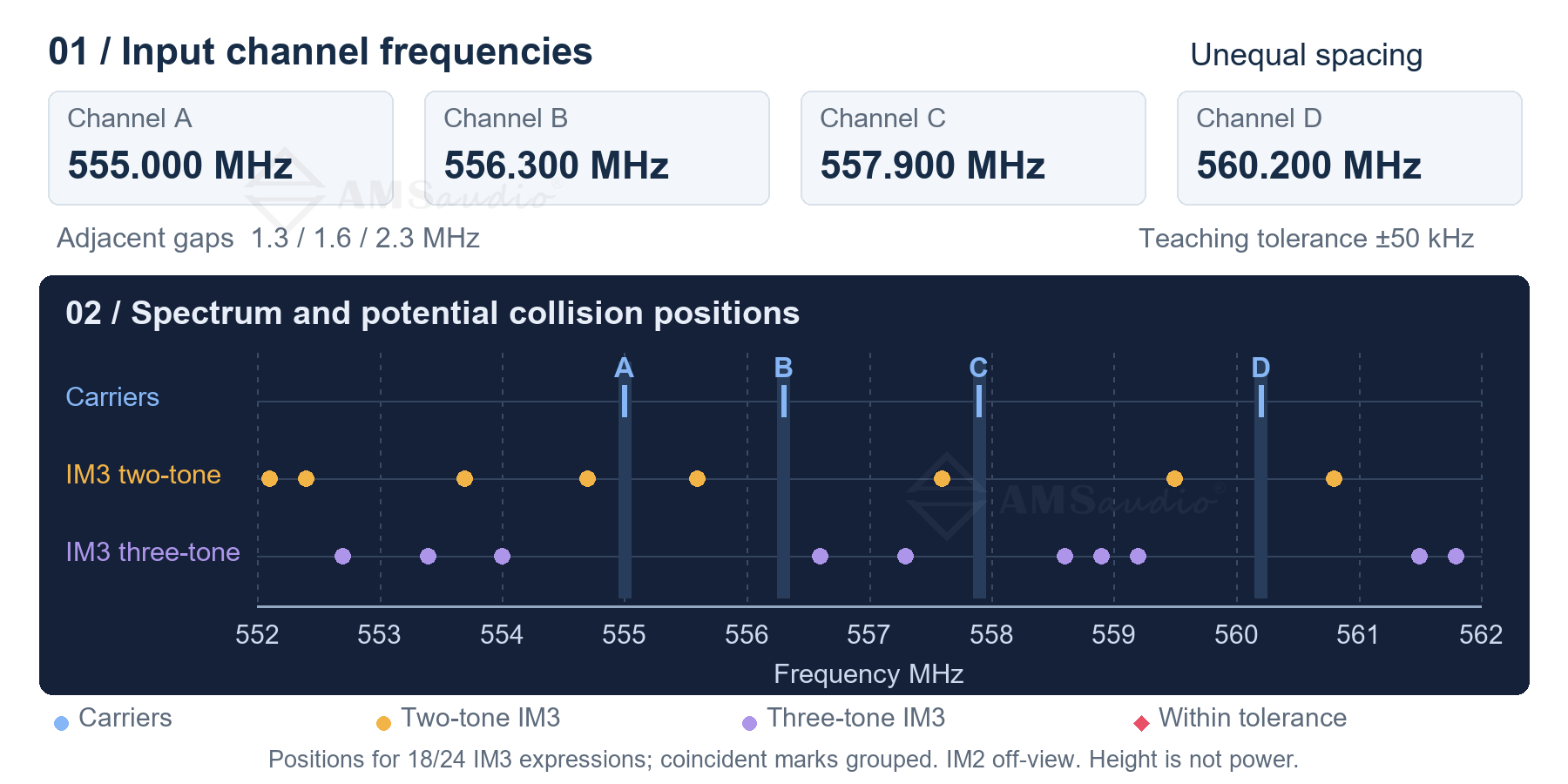
Figure 3  Unequally spaced inputs and potential collision positions

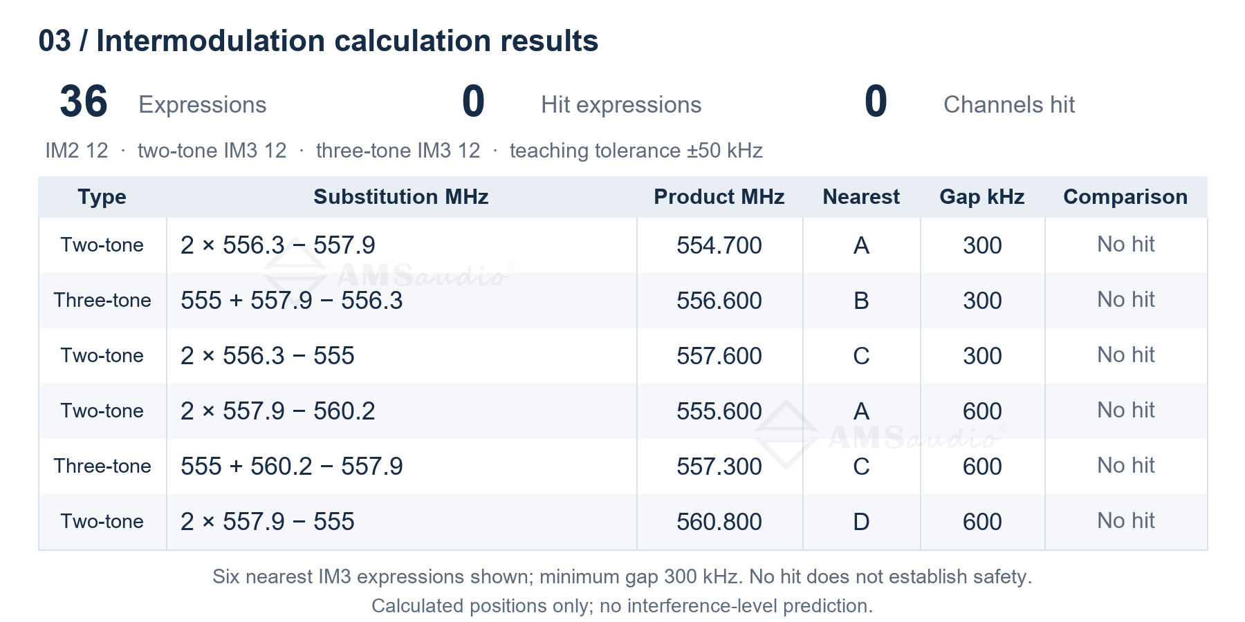
Figure 4  Nearest-channel gaps and results for unequal spacing

This group also produces 36 expressions, with no hits at the ±50 kHz teaching tolerance. The original 2×B−A expression now gives 557.6 MHz, 300 kHz from C at 557.9 MHz. A+C−B gives 556.6 MHz, also 300 kHz from B. Figure 4 shows key results ranked by nearest-channel separation. Across this group's calculated third-order difference products, the minimum separation from a working channel is 300 kHz.

Second order has not been omitted from the calculation. For 555 and 556 MHz, the difference is 1 MHz and the sum is 1111 MHz, both outside this local UHF view. They therefore do not appear in the near-channel plot. No red markers means that the calculated items did not enter the chosen tolerance; it does not establish a deployable, interference-free group.

Use this comparison method when reviewing candidate groups on site. Obtain a current scan and coordinate with accurate equipment models, frequency bands and tuning steps. Recalculate the complete combination after changing a channel, rather than checking only the microphone that moved. Deploy a suitable coordinated plan, then monitor audio and walk the actual routes with all equipment intended to operate simultaneously.

3 Use fine tuning steps and automatic scanning to adjust frequencies

Start with AF and RF. AF shows the audio level; RF shows the received RF signal strength. Watch AF as you speak and check the RF indication before following the frequency-setting steps below.

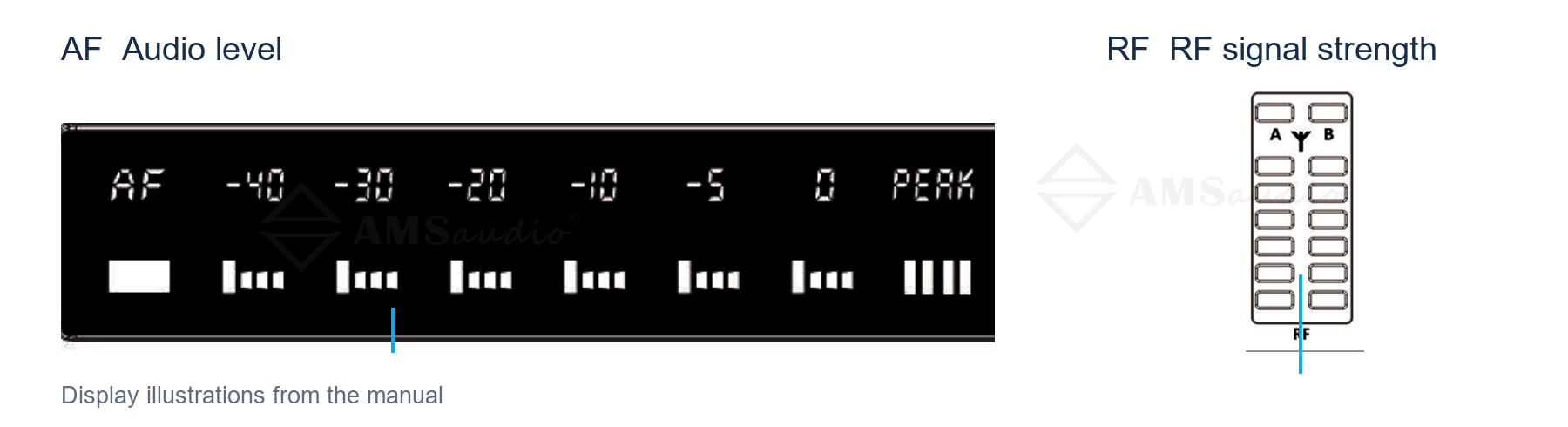
Figure 5  AF and RF indication locations on TC2200

When a frequency combination needs adjustment, AMSaudio TC2200's fine 25 kHz tuning step provides more precise placement options. A 25 kHz step equals 0.025 MHz, so 1 MHz contains 40 increments. Moving from 556.300 to 556.325 MHz is one step; adjustments need not be limited to whole MHz. The step defines the tuning grid, while the required separation between working channels comes from the equipment's coordination requirements.

One-button automatic scanning supports fast frequency selection. TC2200's one-button frequency-planning function can quickly set the receiver to a channel with comparatively less interference, reducing point-by-point manual searching. Follow the operating procedure: hold SYNC to start the scan, then align the transmitter and receiver infrared windows after scanning to complete synchronization. This carries the new channel setting through to both ends of the link.

For a multichannel setup, configure non-TC wireless microphones first. Then scan and synchronize TC systems sequentially, keeping configured transmitters operating normally. During setup, keep transmitters more than 2 metres from receive antennas. Fine steps help implement the selected frequency, while automatic scanning speeds up on-site setting; both make channel rearrangement more convenient for the operator.

Finish by retesting the actual operating positions and saving the final channel list. The frequency calculation, equipment settings and field validation can then be checked against one another.

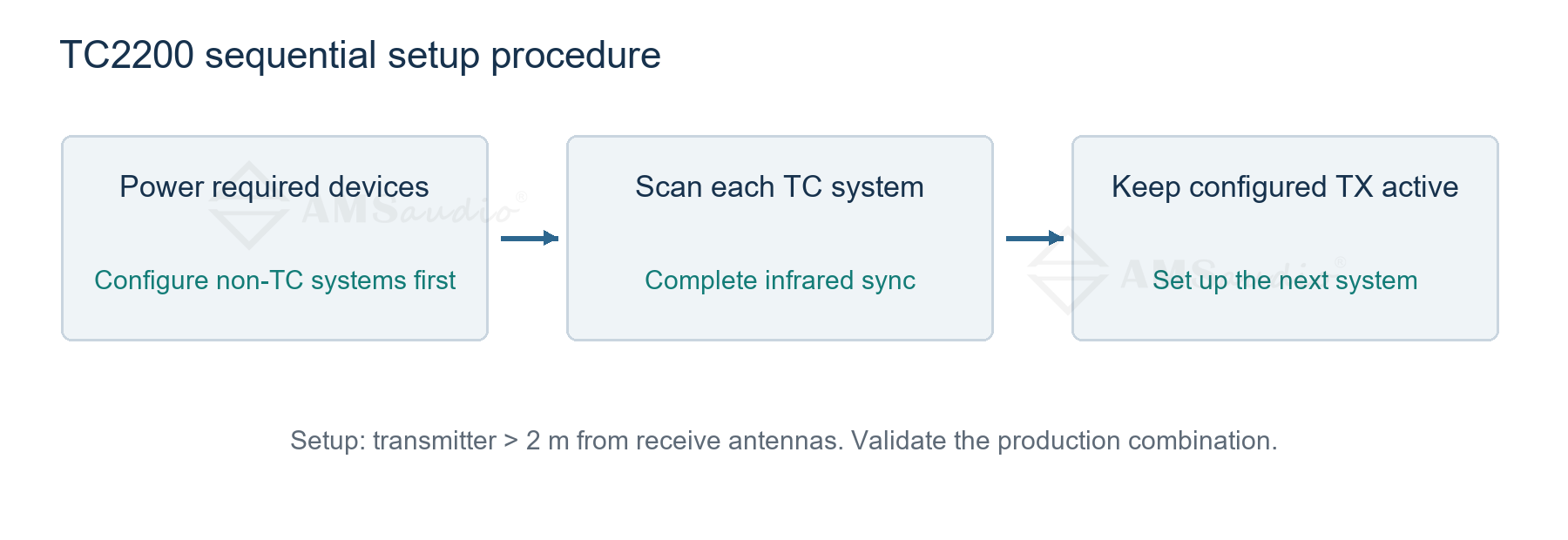
Figure 6  TC2200 sequential scanning and infrared synchronization

#WirelessAudio #RFCoordination #LiveSound